In their article Cramer et al. (2016) propose a theory that explains the difference in vulnerability of MD between individuals. Their model is built on the idea that the strength of the connections between different symptoms differs between individuals. This means that a person can experience fatigue after several sleepless nights, while another person already experiences fatigue after one sleepless night. This network can be seen as a game of dominoes, where strongly connected networks are like domino tiles that are close to each other; one tile tipping makes other tiles tip over as well. Weak connections are like tiles placed far apart; when one tile tips over, it does not necessarily cause other tiles to tip over as well.
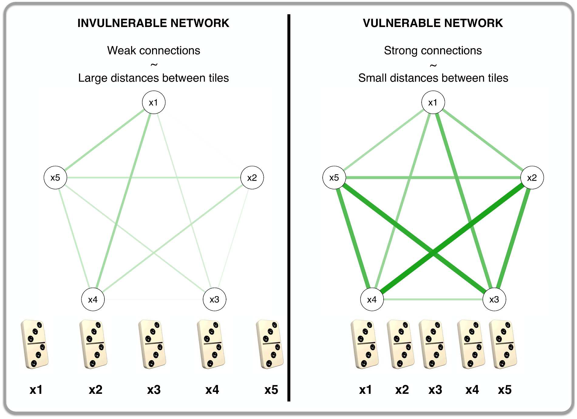 The analogy between vulnerability in a network and spacing of domino tiles (obtained from Cramer et al. (2016))
The model was studied in two parts. The first simulation focussed on the influence of increasing connectivity on the behavior of the MD system. Cramer et al. (2016) tried to answer the question if a system with stronger connections is more prone to end up in a despressed state than a systems with relatively weak connections. The second simulation examined the influence of stress on the behavior of the networks.
Simulation I: The vulnerability hypothesis
For the first simulation, an intra-individual MD model was constructed, which developed over time. In this model, symptoms can be either on (active) or off (inactive). The probability of a symptom becoming active depends on both its threshold and weight parameters. Each symptom has a threshold, which represents the symptoms 'preference' to be active or inactive. A threshold of 0 means that the symptom has no preference, while a positive threshold means the symptom prefers to be active (and a negative threshold represents a preference for being inactive). The weights represent the undirected connections between two symptoms. If the weight is 0, there is no connection. The higher the value of the weight, the more the two corresponding symptoms prefer to be in the same state (on or off). Together, the threshold and weights influence the probability that a symptom becomes active at a particular point in time. The lower its threshold, and the more activation it recieves from its neighbors, the higher the probability the symptom becomes active itself.
The figure below represents the weights between two nodes. The darker a tile, the higher the value of the weight. The exact values of the weights can be found when you hover over the tiles. Pink tiles mean that the symptoms have a negative influence on each other.
This first model is constructed in the following way:
- It is assumed that the total amount of activation symptom i receives at time t is the weighted summation of all neighboring symptoms X. This is represented by the total activation function:
Ait = ∑Jj = 1 WijXjt-1
- The probability that a symptom becomes active at time t depends on the difference between the total activation of its neighbors and the symptom threshold. The parameter bi denotes the absolute value of the thresholds. The higher the total activation exceeds the threshold of that symptom, the higher the probability that the symptom becomes active. This is represented by the probability function:
P (Xit = 1) = 1 ∕ (1 + e(bi - Ait))
The simulation I study
To investigate the differences in vulnerability between strongly and weakly connected networks, the activation function is modified. The connectivity of the system is represented by the connectivity parameter c, which is multiplied with the weights matrix W. This results in the following total activation function:
Ait = ∑Jj = 1 cWijXjt-1
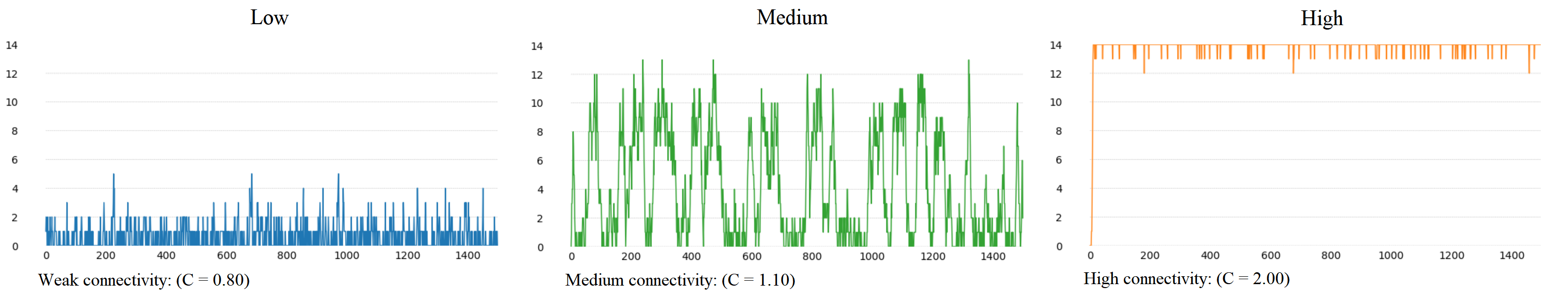
In the article, the connectivity parameter c has three different values, in order to create three different networks: a weak (c = 0.80), a medium (c = 1.10) and a strongly connected network (c = 2.00). We used c in the range 0.5 - 3.0 with these values as anchor points. For all networks, the simulation started with all symptoms in an inactive state. The simulation was run for 10000 time steps and at each time step the total activation and the probability of symptom activation was calculated. From these probabilities, the symptom values for the next time step were sampled.
At each time point, the total number of activated symptoms was tracked, and labelled as D (the state of the system). The more symptoms were active, the more 'depressed' the system was. Later, in above and beyond we specify this further.
As the graphs below show, 'depressed' states increase with connectivity. For a weakly connected system (c < 1.0) there are moments where several sympoms occur, but the system never develops into a 'depressed' one. As connecitivity increases, the system starts to oscillate between the 'non-depressed' and 'depressed' state. The system is able to go back to a 'non-depressed' state without changes to the network (in the real world, that would be therapy or medication). The strongly connected network (c > 1.2 ) becomes 'depressed' after a short time, and does not change back to the 'non-depressed' state. This can be regarded as a person that will not be able to get out of a depression without external help.
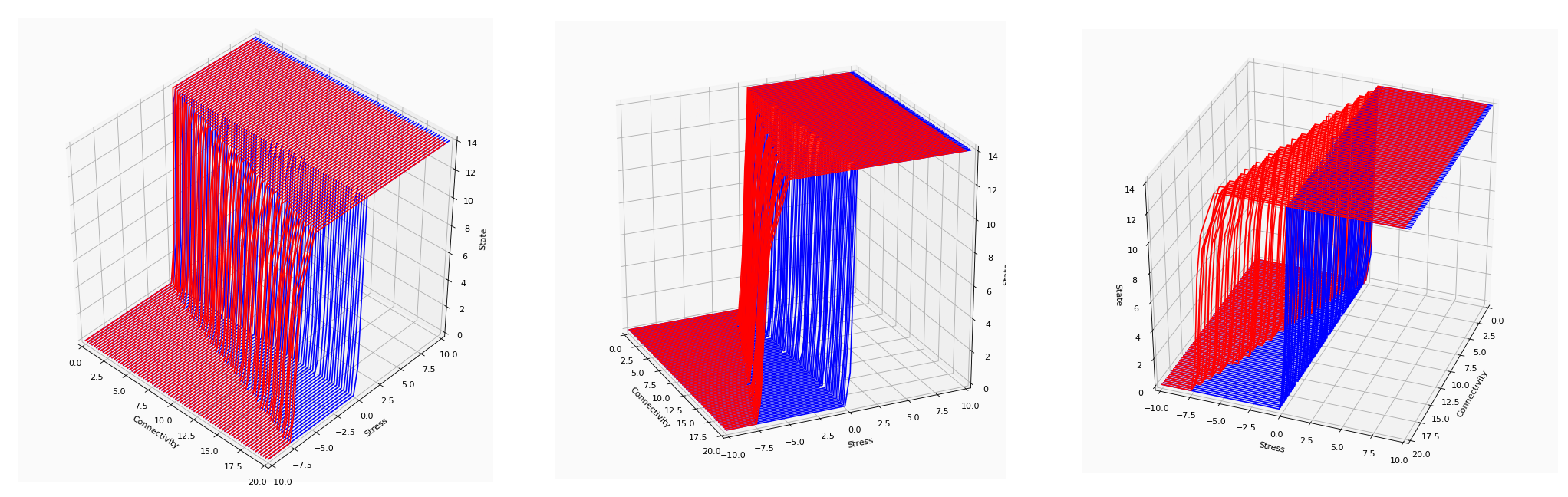
 The state of the MD system in response to stress for varying connectivity
Interactive Simulation I
To get a feeling of the behaviour of the system, play around with the c-parameter and the number of iterations. Don't forget to press Update Graph!
The model used in simulation I represents the development of MD without an external trigger. To include the influence of externel events, a second simulation was done.
Simulation II: Investigating the influence of external stress on the MD systems
Since external stressful events (like the death of a loved one) have an impact on the development of MD, the simulation study above does not do justice to real life. In this second simulation study, there is an additional factor influencing the MD network: stress. The aim of this addition is to try to answer the following question:
What happens to systems with increasing connectivity, when external stress is added?
To answer this question, the total activation function was modified into the following equation:
Ait = ∑Jj = 1 cWijXjt-1 + Sit
For the sake of simplicity, it was assumed that stress influences all symptoms equally. Stress was first increased from -15 to 15, then decreased from 15 to -15 with small steps. The system changes from a 'non-depressed' state to a 'depressed' state in response to increasing stress (the blue lines). For a weakly connected network in a 'depressed' state, decreasing the stress level makes it switch back to a 'non-depressed' state at the initial tipping point on which it switched to a 'depressed' state in the first place (see the red lines). For a heavilly connected network, this tipping point lays after the initial tipping point. So, to get into a 'depressed' state a different level of stress is needed, than to get out again. For someone with a heavily connected network to get out of this 'depressed' state, a lower amount of stress is needed, than the initial tipping point. In the graph you see, for a weakly connected network, that going to a 'depressed' state happens at the same stress level as going back to a 'non-depressed' state, while a network which is heavily connected needs a lower stress level to switch back to a 'non-depressed' state.
Interactive Simulation II
The graph below lets you play with this system. Increase or decrease the conncectivity and see what happens. Don't forget c = 0.8 is a weakly connected network, c = 1.1 is a medium connected network and c = 2 is a heavily connected network.